Using Business Description for a Firm-Level Estimate of Greeness
Contents
Using Business Description for a Firm-Level Estimate of Greeness#
Alessi and Battiston (2022) [AB22] propose a top-down approach to measure firm greeness, by computing a taxonomy alignment coefficient with data at sector level (NACE sectors).
As we want to estimate a firm level measure of greeness, we develop a text-mining approach. More specifically, we define the firm-level exposure to a given activity as the semantic similarity between the business description of the firm and the description of the activity.
In this part, we will first explain the Natural Language Processing approach we develop to measure firm-level greeness and then discuss the results.
Embeddings with a Sentence Transformer Model#
We first need to transform the business description and activities descriptiom from our taxonomy from unstructured data (text) into a numerical representation. To do so, we use a Sentence Transformer model to create numerical vector representation of the meanings of the business description of the firm \(i\), \(D_{i}\) and the description of the activity \(k\), \(A_{k}\):
and
Where \(Emb^{D_{i}}\) and \(Emb^{A_k}\) are the numerical vector representation (embeddings) of \(D_{i}\) and \(A_{k}\), performed with the Sentence Transformer model \(ST()\).
Cosine Similarity#
We want to be able to determine if the business description \(D_{i}\) is related to one of the activity defined in our taxonomy.
As we now have numerical vector representations \(Emb^{D_{i}}\) and \(Emb^{A_k}\), we can apply principles from semantic search by determining the closeness of our two vectors. Recalling that dimensions of our vector representation relate to the underlying meaning of the text, computing the closeness of our vectors allows for determining the semantic similarity between our descriptions.
One way to do so is by computing the cosine similarity between our two vectors. The cosine similarity measures the cosine of the angle of those two vectors. The closer the cosine similarity to 1 is, the more related the descriptions are:
For each business description, the cosine similarity is computed against each activity description in our taxonomy. The maximum cosine similarity measure is retained, with the associated activity.
Greeness Measure#
Finally, we adopt the following rule to attribute a greeness score to each issuer:
If \(cos(\theta_{D_{i},k}) \leq 0.5\), a 0 score is attributed to the issuer.
If the activity \(k\) for which the cosine similarity with the business description was the highest is among the brown activities in our taxonomy, a score of \(-cos(\theta_{D_{i},k})\) is attributed. A score of \(cos(\theta_{D_{i},k})\) is attributed if the activity is among the green activities in our taxonomy.
Python Implementation & Results#
Below is the Python code for determining the greeness measure, using data in the materials folder.
We first load the file containing the descriptions for the green and brown activities:
import pandas as pd

# our taxonomy
taxo = pd.read_excel('Green_Taxo.xlsx')

# definitions of green and brown activities
green_definitions = taxo[taxo['Type']=='Green'].Description.tolist()

brown_definitions = taxo[taxo['Type'] == 'Brown'].Description.tolist()
We then load the data containing the business description. We drop the rows without business description or with too short business description (web-scrapping is an art rather than a science…):
business_desc = pd.read_csv('sandp_business_desc.csv')

business_desc.dropna(inplace = True)
mask = (business_desc['Business_description'].str.len() >= 100)
business_desc = business_desc.loc[mask]
list_D = business_desc['Business_description'].tolist()
Then we use the sentence-transformers package for embedding our descriptions. Please install it if needed with:
pip install sentence_transformers
Once installed, we can then proceed to the embedding step for the activities description:
from sentence_transformers import SentenceTransformer, util
import torch

ST = SentenceTransformer('paraphrase-mpnet-base-v2')
emb_A = ST.encode(taxo.Description.tolist(), convert_to_tensor = True)
We create the following function to get the greeness score for each row in our dataframe:
def get_exposure(business_desc:str, emb_A:list, taxo:pd.DataFrame):
  emb_desc = ST.encode([business_desc], convert_to_tensor=True)
  result = util.semantic_search(emb_desc, emb_A, top_k = 1)[0][0]
  if (taxo.iloc[result['corpus_id']]['Type'] == 'Brown') & (result['score'] > 0.5):
    exposure = - result['score']
  elif (taxo.iloc[result['corpus_id']]['Type'] == 'Green') & (result['score'] > 0.5):
    exposure = result['score']

  else:
    exposure = 0.0
  return exposure

business_desc['Greeness'] = business_desc.apply(lambda x: get_exposure(business_desc = x['Business_description'],
                                                         emb_A = emb_A,
                                                         taxo = taxo), axis = 1)
Let’s plot the results for non-neutral firms:
import seaborn as sns
import matplotlib.pyplot as plt
import plotly.express as px

results = business_desc[business_desc['Greeness'] != 0]
results = results.sort_values(by = 'Greeness', ascending = False)

f , ax = plt.subplots(figsize=(10, 10))

g = sns.barplot(data = results,
            ax = ax,
            x = 'Security',
            y = 'Greeness')

g.set_xticklabels(
    labels=results.Security.tolist(),
    rotation=90)

plt.show()
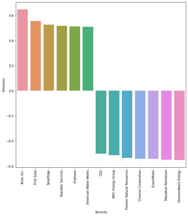
Figure: Greeness Measure#
A few firms among the S&P universe are targeted as green or brown with our greeness measure. This can be explained by the fact that measuring firms greeness with the business description and a quite stringent cosine similarity threshold is equivalent to looking for pure-players in green technologies which limits the universe.
This underlines the narrow investable green securities universe for the time being.
Obtaining more granular results would involves applying the approach of identifying green and brown activities at the business segment level, in order to obtain a measure close to the green intensity measure used by Roncalli et al. (2022) [IMNT22].