Transition Portfolio#

In what follows we present our simple framework for the construction of a portfolio with a dual objective:

Minimizing the tracking error volatility risk and
Improving the greeness of the portfolio version compared to the benchmark.

To do so, we follow the approach from Roncalli (2023) [Ron23], formulating our tilting problem as a portfolio optimization with the presence of a benchmark.

In this part, we first define benchmark greeness, excess greeness and tracking error volatility, before discussing the construction of a transition portfolio and the trade-off involved in targeting portfolio’s greeness improvement.

Benchmark Greeness#

We need first to define the benchmark greeness. Let’s assume \(b\) the vector of weights of the benchmark which is equally-weighted.

Let’s assume \(G\) a vector of greeness measure of the stocks composing the benchmark.

The benchmark greeness can be computed as:

(1)#\[\begin{equation} G(b) = b^TG \end{equation}\]

Below is the Python code to load the data in the materials folder:

import pandas as pd

greeness = pd.read_csv('results_greeness.csv')
data_fin = pd.read_csv('data_fin.csv')

df = greeness.merge(data_fin, how = 'inner', on = 'Ticker').dropna()

list_entities = df.Ticker.drop_duplicates().tolist()
greeness_score = greeness[greeness['Ticker'].isin(list_entities)].Greeness.tolist()

Below is the Python code for computing the benchmark greeness:

import numpy as np
b = np.array([ 1 / len(list_entities)] * len(list_entities))

G = np.array(greeness_score)

np.dot(b, G)

Portfolio’s Excess Greeness and Tracking Error#

Having the previous benchmark, let’s assume a portfolio with the same issuers than the benchmark, but with different weights \(x\).

x = np.random.dirichlet(np.ones(len(greeness_score)),size=1)[0]

We define the excess greeness of our portfolio, that is the positive or negative deviation from our benchmark greeness:

(2)#\[\begin{equation} G(x|b) = (x - b)^T G \end{equation}\]

Below is the code to compute the excess greeness of our portfolio:

excess_greeness = (x - b).T @ G

We can also compare the relative performance of the portfolio compared to the benchmark with the tracking error volatility:

(3)#\[\begin{equation} \sigma(x|b) = \sqrt{(x - b)^T \Sigma (x - b)} \end{equation}\]

Below we compute the tracking error volatility:

Sigma = df.pivot(index = 'Date', columns = 'Ticker', values = 'Return').fillna(0).cov().reset_index(drop=True).to_numpy()
te = np.sqrt((x - b).T @ Sigma @ (x - b))

Transition Investing Objectives#

In the previous example, we compared the greeness performance of a portfolio against a benchmark, with predefined portfolio’s weights.

However, the objective of investors is to improve the portfolio’s greeness while controlling the tracking error volatility.

Denoting \(\gamma\) as the risk tolerance parameter, we have the following optimization problem:

\[\begin{equation*} \begin{aligned} & x^* = & & argmin \frac{1}{2} \sigma^2 (x |b) - \gamma G (x | b) \\ & \text{subject to} & & 1_n^Tx = 1, \\ &&& 0_n \leq x \leq 1_n. \end{aligned} \end{equation*}\]

Where the constraints simply mean that the sum of the resulting weights \(x\) need to be 1 and that individual weights \(x_i\) need to between 0 and 1.

Varying the parameter value of \(\gamma\) gives you the efficient frontier of tracking a benchmark with a greeness objective.

Below we install and import the qpsolvers package and formulate the QP problem of the optimization:

from qpsolvers import solve_qp

def portfolio_tilting(Sigma, G, b, gamma):
  """QP formulation"""
  
  P = Sigma # Q 
  q = - (gamma * G + Sigma @ b) # R, minus because we want to maximize it!
  A = np.ones(len(G)).T # A
  b = np.array([1.]) # B
  lb = np.zeros(len(G))
  ub = np.ones(len(G))
  x = solve_qp(P = P,
               q = q,
               A = A, 
               b = b,
               lb = lb,
               ub = ub,
               solver = 'osqp')
  
  return x


def get_perf_tilting(x, b, Sigma, G):
  excess_greeness = (x - b).T @ G
  te = np.sqrt((x - b).T @ Sigma @ (x - b))
  return excess_greeness, te

Targeting a Specific Greeness Improvement#

We will now target a specific portfolio greeness improvement and see the resulting portfolio’s weights.

To do so, one can use the bisection algorithm.

import numpy as np

def bisection(f, a, b, tol): 
    # approximates a root, R, of f bounded 
    # by a and b to within tolerance 
    # | f(m) | < tol with m the midpoint 
    # between a and b Recursive implementation
    
    # check if a and b bound a root
    if np.sign(f(a)) == np.sign(f(b)):
        raise Exception(
         "The scalars a and b do not bound a root")
        
    # get midpoint
    m = (a + b)/2
    
    if np.abs(f(m)) < tol:
        # stopping condition, report m as root
        return m
    elif np.sign(f(a)) == np.sign(f(m)):
        # case where m is an improvement on a. 
        # Make recursive call with a = m
        return bisection(f, m, b, tol)
    elif np.sign(f(b)) == np.sign(f(m)):
        # case where m is an improvement on b. 
        # Make recursive call with b = m
        return bisection(f, a, m, tol)

def greeness_targeting(Sigma, G, b, target_excess_score):
  f = lambda x: (portfolio_tilting(Sigma = Sigma,
                        G = G,
                        b = b,
                        gamma = x) - b).T @ G - target_excess_score
    
  x_star_greeness = portfolio_tilting(Sigma = Sigma,
                        G = G,
                        b = b,
                        gamma = bisection(f, 0, 0.2, 0.01))
  return x_star_greeness

Let’s test with a target improvement of 10%:

x_star_greeness = greeness_targeting(Sigma = Sigma,
                                     G = G,
                                     b = b,
                                     target_excess_score = 0.1)

And let’s plot the resulting top 15 securities in terms of weights deviation from the benchmark:

results_target = pd.DataFrame({"Ticker":list_entities,
                               "Security":df.Security.drop_duplicates().tolist(),
                               "Tilted_Weights":x_star_greeness, "Initial_Weights":b.tolist()})
results_target['Deviation'] = results_target['Tilted_Weights'] - results_target['Initial_Weights']

import seaborn as sns                    # This is one library for plotting
import matplotlib.pyplot as plt          # Yet another library for visualization
import plotly.express as px   

results_target = results_target.sort_values(by = 'Deviation', ascending = False)

top_15 = results_target.sort_values(by = 'Deviation', ascending = False).head(15)

f , ax = plt.subplots(figsize=(10, 10))

g = sns.barplot(data = top_15,
            ax = ax,
            x = 'Security',
            y = 'Deviation')

g.set_xticklabels(
    labels=top_15.Security.tolist(),
    rotation=90)

plt.show()

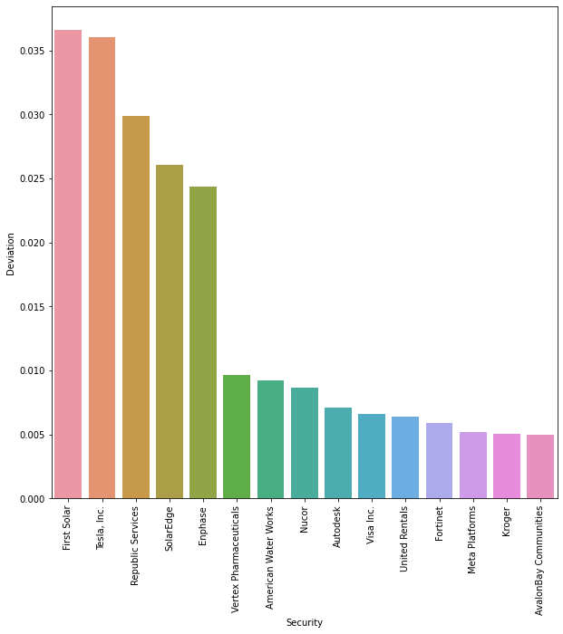
_images/weights_dev.png — Figure: Top 15 securities in terms of weights deviation from the benchmark#

With a targeted excess greeness score of 10%, we can see that the properties of our transition portfolio follows the expected behavior of our mixed green-brown taxonomy:

The securities with the highest exposure to greeness (ie. the pure-players) are the ones with the highest positive weights deviation
The neutral securities follow the greenest ones, replacing the brown securities in the portfolio.

However, we need to investigate the cost associated with this greeness improvement, noteworthy knowing the narrow universe of green investments.

TE and Excess Greeness Trade-Off#

We can measure the cost of deviation from the initial benchmark with the tracking error. We can test the properties of our transition metrics by testing the cost associated with various levels of greeness improvement.

Below is the Python code to compute the tracking error for various levels of greeness excess:

list_targets = [0.1, 0.2, 0.3, 0.4 , 0.5]

list_te = []

for target in list_targets:
  x_star_greeness = greeness_targeting(Sigma = Sigma,
                                     G = G,
                                     b = b,
                                     target_excess_score = target)
  excess_greeness, te = get_perf_tilting(x = x_star_greeness, 
                                       b = b, 
                                       Sigma = Sigma,
                                       G = G)
  
  list_te.append(te)

f , ax = plt.subplots(figsize=(10, 10))

g = sns.barplot(
            ax = ax,
            x = np.array(list_targets) * 100,
            y = np.array(list_te) * 100)
plt.xlabel("Excess Greeness Target (in %)")
plt.ylabel("TE Volatility (in %)")
plt.show()

Below is a chart showing the increase of tracking error as we increase the excess greeness target.

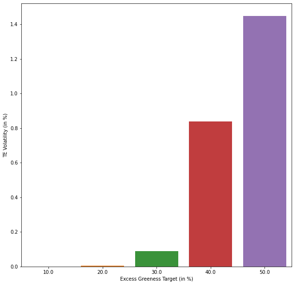
_images/arbitrage.png — Figure: TE Volatility vs. Excess Greeness Targets#

A low level of targeted improvement leads to small tracking error, because from 10 to 30% of excess greeness target, the investment universe is still large, spanning green and neutral activities. However, exceeding 30% of excess greeness target leads to important tracking error, as the investment universe shrinks to the narrow green activities pure-players universe.

Climate Investing with NLP 0 documentation

Transition Portfolio

Contents